3. Using AIMBAT

3.1. Seismic Analysis Code (SAC)

AIMBAT uses Seismic Analysis Code (SAC) formatting for some of the files it runs and outputs. To get SAC, you will need to fill out a software request form available on the IRIS website.

3.2. SAC Input/Output procedures for AIMBAT

Aimbat converts SAC files to python pickle data structure to increase data processing efficiency by avoiding frequent SAC file I/O.

Reading and writing SAC files is done only once each before and after data processing, and intermediate processing is performed on python objects and pickles.

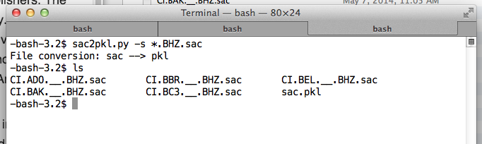
3.2.1. Converting from SAC to PKL files

Place the SAC files you want to convert to a pickle (PKL) file into the same folder. Suppose, for instance, they are BHZ channels. Note that the SAC files must be of the same channel. cd into that folder, and run:

aimbat-sac2pkl -s *.BHZ.sac

The output should be a PKL file in the same folder as the sac files.

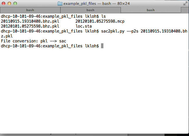
3.2.2. Converting from PKL to SAC files

cd into the folder containing the PKL file that you wish to convert into SAC files, and run:

aimbat-sac2pkl --p2s <name-of-file>.pkl

The SAC files contained within will output into the same folder as the PKL file is stored in.

3.3. Parameter Configuration

3.3.1. Backend

Matplotlib works with six GUI (Graphical User Interface) toolkits:

WX
Tk
Qt(4)
FTK
Fltk
macosx

The GUI of AIMBAT uses the following to support interactive plotting:

Visit these pages for an explanation of the backend and how to customize it.

AIMBAT uses the default toolkit Tk and backend TkAgg.

In the latest version, user does not need to setup the backend for the SAC plotting functions.

3.3.2. Configuration File

Parameters for the package can be set up by a configuration file ttdefaults.conf, which is interpreted by the module ConfigParser. This configuration file is searched in the following order:

file ttdefaults.conf in the current working directory
file .aimbat/ttdefaults.conf in your HOME directory
a file specified by environment variable TTCONFIG
file ttdefaults.conf in the directory where AIMBAT is installed

Python scripts in the <pkg-install-dir>/pysmo-aimbat-0.1.2/scripts can be executed from the command line. The command line arguments are parsed by the optparse module to improve the scripts’ exitability. If conflicts existed, the command line options override the default parameters given in the configuration file ttdefaults.conf. Run the scripts with the -h option for the usage messages.

3.3.2.1. Example of AIMBAT configuration file ttdefaults.conf

ttdefaults.conf	Description
[sacplot]
colorwave = blue	Color of waveform
colorwavedel = gray	Color of waveform which is deselected
colortwfill = green	Color of time window fill
colortwsele = red	Color of time window selection
alphatwfill = 0.2	Transparency of time window fill
alphatwsele = 0.6	Transparency of time window selection
npick = 6	Number of time picks (plot picks: t0-t5)
pickcolors = kmrcgyb	Colors of time picks
pickstyles	Line styles of time picks (use second one if ran out of color)
figsize = 8 10	Figure size for plotphase.py
rectseis = 0.1 0.06 0.76 0.9	Axes rectangle size within the figure
minspan = 5	Minimum sample points for SpanSelector to select time window
srate = -1	Sample rate for loading SAC data. Read from first file if srate < 0

[sachdrs]
twhdrs = user8 user9	SAC headers for time window beginning and ending
ichdrs = t0 t1 t2	SAC headers for ICCS time picks
mchdrs = t2 t3	SAC headers for MCCC input and output time picks
hdrsel = kuser0	SAC header for seismogram selection status
qfactors = ccc snr coh	Quality factors: cross-correlation coefficient, signal-to-noise ratio, time domain coherence
qheaders = user0 user1 user2	SAC Headers for quality factors
qweights = 0.3333 0.3333 0.3333	Weights for quality factors

[iccs] or Align/Refine
srate = -1	Sample rate for loading SAC data. Read from first file if srate < 0
xcorr_modu = xcorrf90	Module for calculating cross-correlation: xcorr for Numpy or xcorrf90 for Fortran
xcorr_func = xcorr_fast	Function for calculating cross-correlation: xcorr_full/fast/faster, reverse polarity allowed xcorr_full/fast/faster_polarity, reverse polarity not allowed
shift = 10	Sample shift for running coarse cross-correlation
maxiter = 10	Maximum number of iteration
convepsi = 0.001	Convergence criterion: epsilon
convtype = coef	Type of convergence criterion: coef for correlation coefficient, or resi for residual
stackwgt = coef	Weight each trace when calculating array stack
fstack = fstack.sac	SAC file name for the array stack

[mccc]
srate = -1	Sample rate for loading SAC data. Read from first file if srate \(< 0\)
ofilename = mc	Output file name of MCCC.
xcorr_modu = xcorrf90	Module for calculating cross-correlation: xcorr for Numpy or xcorrf90 for Fortran
xcorr_func = xcorr_fast	Function for calculating cross-correlation: xcorr_full/fast/faster, reverse polarity allowed xcorr_full/fast/faster_polarity, reverse polarity not allowed
shift = 10	Sample shift for running coarse cross-correlation
extraweight = 1000	Weight for the zero-mean equation in MCCC weighted lsqr solution
lsqr = nowe	Type of lsqr solution: no weight
#lsqr = lnco	Type of lsqr solution: weighted by correlation coefficient, solved by lapack
#lsqr = lnre	Type of lsqr solution: weighted by residual, solved by lapack
rcfile = .mcccrc	Configuration file for MCCC parameters (deprecated)
evlist = event.list	File for event hypocenter and origin time (deprecated)

signal
tapertype = hanning	Taper type
taperwidth = 0.1	Taper width
fhdrBand = kuser1	SAC Header to store filter type
fhdrApply = kuser1	SAC Header to store applying filter or not
fhdrRevPass = user4	SAC Header to store reverse pass of filter
fhdrLowFreq = user5	SAC Header to store low frequency of band pass filter
fhdrHighFreq = user6	SAC Header to store high frequency of band pass filter
fhdrOrder = user7	SAC Header to store order of band pass filter
fvalApply = 0	Value of applying filter or not
fvalBand = bandpass	Value of filter type
fvalRevPass = 0	Value of reverse pass filter
fvalLowFreq = 0.05	Value of low frequency of band pass filter
fvalHighFreq = 2	Value of high frequency of band pass
fvalOrder = 2	Value oforder of band pass filter

3.4. SAC Data Access

NOTE: All .sac files must include origin time, hypocenter, as well as station coordinates and elevation in their headers.

3.4.1. Python Object for SAC File

The pysmo.core.sac package is developed to read and write individual SAC files. The Python class SacIO of module pysmo.core.sac.sacio opens a SAC file and returns an object including data and all SAC header variables as their attributes. Modifications of object attributes are saved to file. It is written purely in Python so that it also runs with Jython.

3.4.1.1. egsac.py

The <pkg-install-dir>/example-scripts/egsac.py script gives a simple example to read, resample, and plot a seismogram using pysmo, Scipy, and Matplotlib. You can type the codes in a Python/iPython shell, or run as a script in the data example directory <pkg-install-dir>/data-example/Event_2011.09.15.19.31.04.080, hereafter referred to as <example-event-dir>.

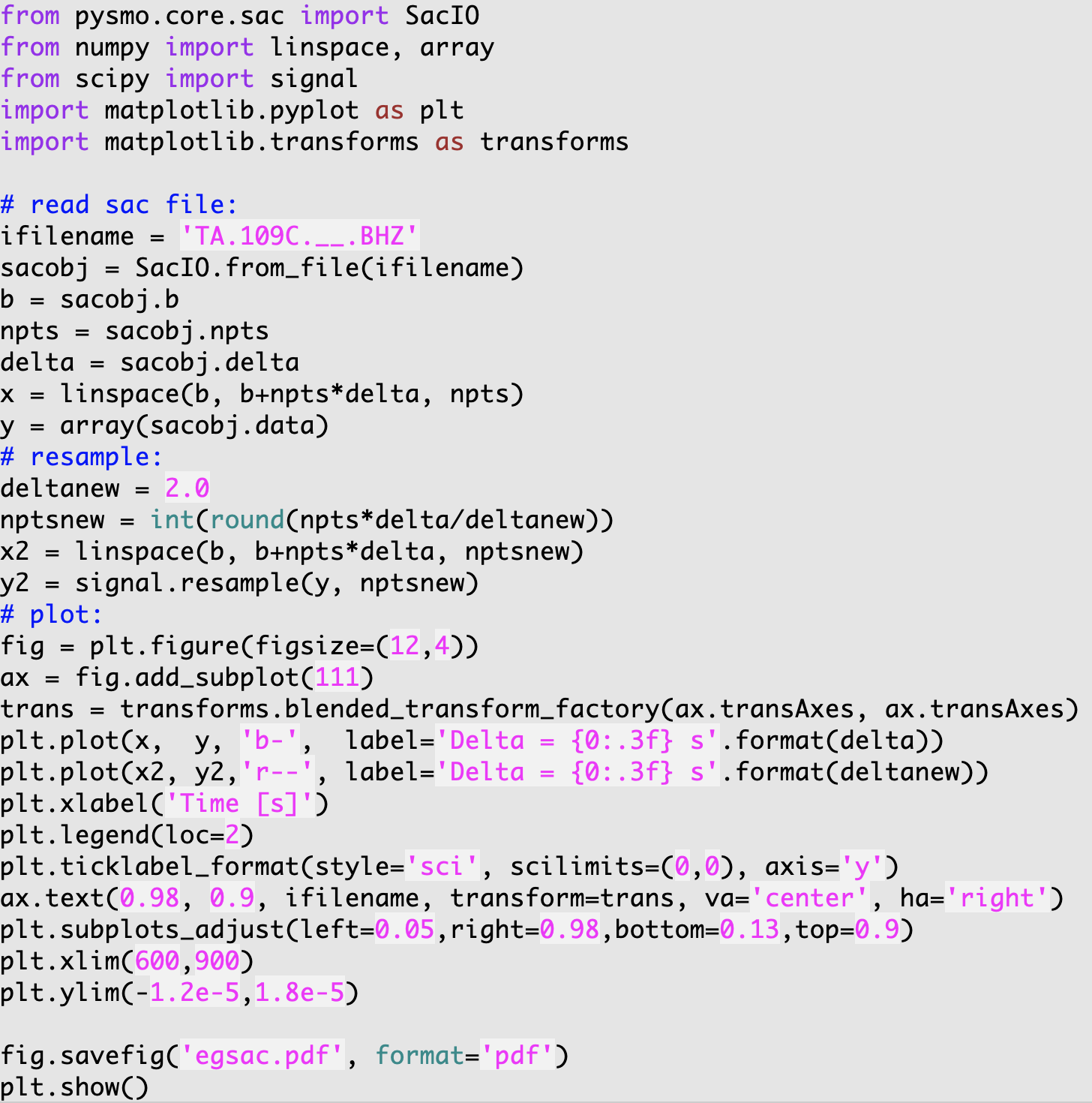
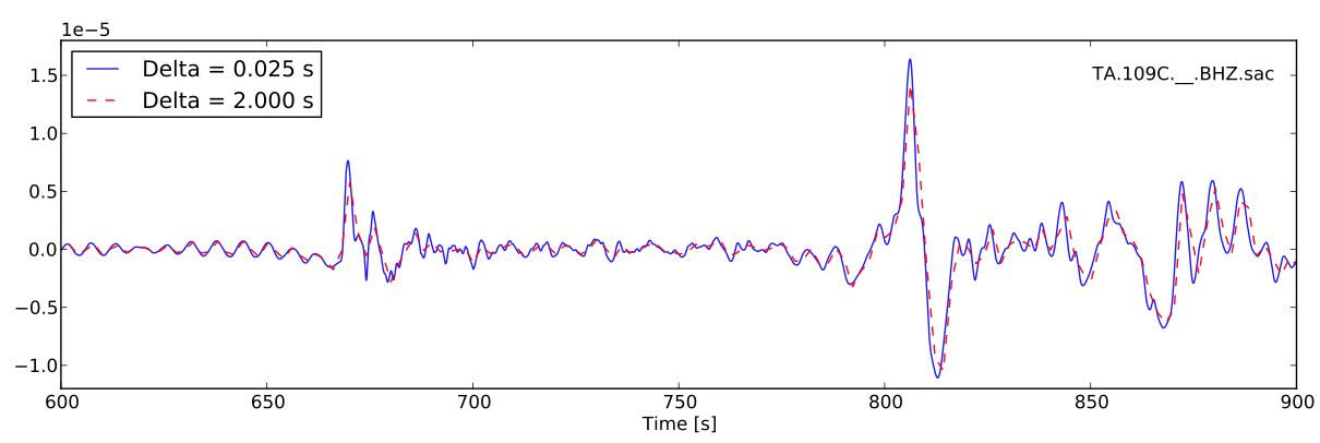
3.4.1.2. Resampling Seismograms

In this example, a SAC file named TA.109C.\_\_.BHZ.sac is read in as a sacfile object. The time array is calculated from SAC headers. The data array is resampled from interval 0.025 to 2.0 seconds using Scipy’s signalprocessing module.

Add the following codes to write the resampled seismogram to file TA.109C.\_\_.BHZ.sac:

sacobj.delta = deltanew
sacobj.npts = nptsnew
sacobj.data = y2

3.4.2. Python Pickle for SAC Files

The pysmo.core.sac.sacio module converts SAC files to SacIO objects. Any modification of the objects are instantly written to files. In data processing, the user may want to abandon changes made earlier, which brings the need of a buffer for the SacIO objects.

The SacDataHdrs class in the pysmo.aimbat.sacpickle module is written on top of pysmo.SacIO to serves this purpose by reading a SAC file and returning a sacdh object that is very similar to the sacfile object. Essentially, the sacdh object is a copy of the sacfile object in the memory, except that SAC headers ‘t0-t9’, ‘user0-user9’, and ‘kuser0-kuser2’ are saved in three Python lists.

A gsac object of the SacGroup class consists of a group of sacdh objects from event-based SAC data files, earthquake hypocenter information, and station locations. An additional step is required to save changes in the gsac object to files.

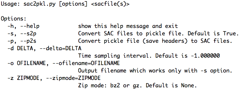
In order to avoid frequent SAC file I/O, the pickle/cPickle module is used for serializing and de-serializing the gsac object structure. Thus the data processing efficiency is improved because reading and writing of SAC files are done only once each before and after data processing. Script aimbat-sac2pkl does the conversions between SAC files and Python pickles.

Its usage message can be printed out by running at command line:

aimbat-sac2pkl -h

and the result is displayed in the figure below. For example, in the data example directory <example-event-dir>, run:

aimbat-sac2pkl -s *Z -o 20110915.19310408.bhz.pkl -d 0.025

to read 163 vertical component seismograms at a sample interval of 0.025 s and convert to a gsac object, which is saved in the pickle file 20110915.19310408.bhz.pkl.

To save disk space, compressed pickle files in gz and bz2 formats can be generated by:

aimbat-sac2pkl -s *Z -o 20110915.19310408.bhz.pkl -d 0.025 -z gz
aimbat-sac2pkl -s *Z -o 20110915.19310408.bhz.pkl -d 0.025 -z bz2

at the cost of more CPU time.

After processing, run:

aimbat-sac2pkl 20110915.19310408.bhz.pkl -p

to convert the pickle file to SAC files.

See the doc string of pysmo.aimbat.sacpickle by typing in a python console:

from pysmo.aimbat import sacpickle
print(sacpickle.\_\_doc\_\_)

and also the documentation on pickle for more information about the Python data structure, pickling, and unpickling.

3.4.3. SAC Plotting and Phase Picking

SAC plotting and phase picking functionalities are replicated and enhanced based on the GUI neutral widgets (such as Button and SpanSelector) and the event (keyboard and mouse events such as key\_press\_event and mouse\_motion\_event handling API of Matplotlib.

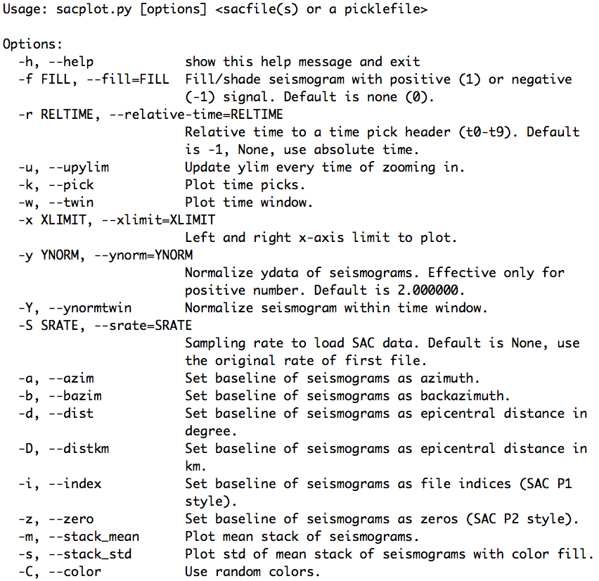
They are implemented in two modules, pysmo.aimbat.plotphase and pysmo.aimbat.pickphase, which are used by corresponding scripts aimbat-sacplot and aimbat-sacppk executable at command line. Their help messages are displayed in the figures below.

3.4.4. SAC Plotting

Options “-i, -z, -d, -a, and -b” of aimbat-sacplot set the seismogram plotting baseline as file index, zero, epicentral distance in degrees, azimuth, and back-azimuth, respectively. The user can run aimbat-sacplot directly with the options, or run individual scripts aimbat-sacp1, aimbat-sacp2, aimbat-sacprs, aimbat-sacpaz, and aimbat-sacpbaz, which preset the baseline options and plot seismograms in SAC p1 style, p2 style, record section, and relative to azimuth and back-azimuth. The following commands are equivalent:

aimbat-sacplot -i, aimbat-sacp1
aimbat-sacplot -z, aimbat-sacp2
aimbat-sacplot -d, aimbat-sacprs
aimbat-sacplot -a, aimbat-sacpaz
aimbat-sacplot -b, aimbat-sacpbaz

Input data files need to be supplied to the scripts in the form of either a list of SAC files or a pickle file that includes multiple SAC files. For example, a bhz.pkl file is generated from 22 vertical component seismograms TA.[1-K]*Z by running:

aimbat-sac2pkl TA.[1-K]*BHZ -o bhz.pkl -d0.025

in the data example directory <example-event-dir>. Then the two commands are equivalent:

aimbat-sacp1 TA.[1-K]*Z

or:

aimbat-sacp1 bhz.pkl

For large numbers of seismograms, the pickle file is suggested because of faster loading.

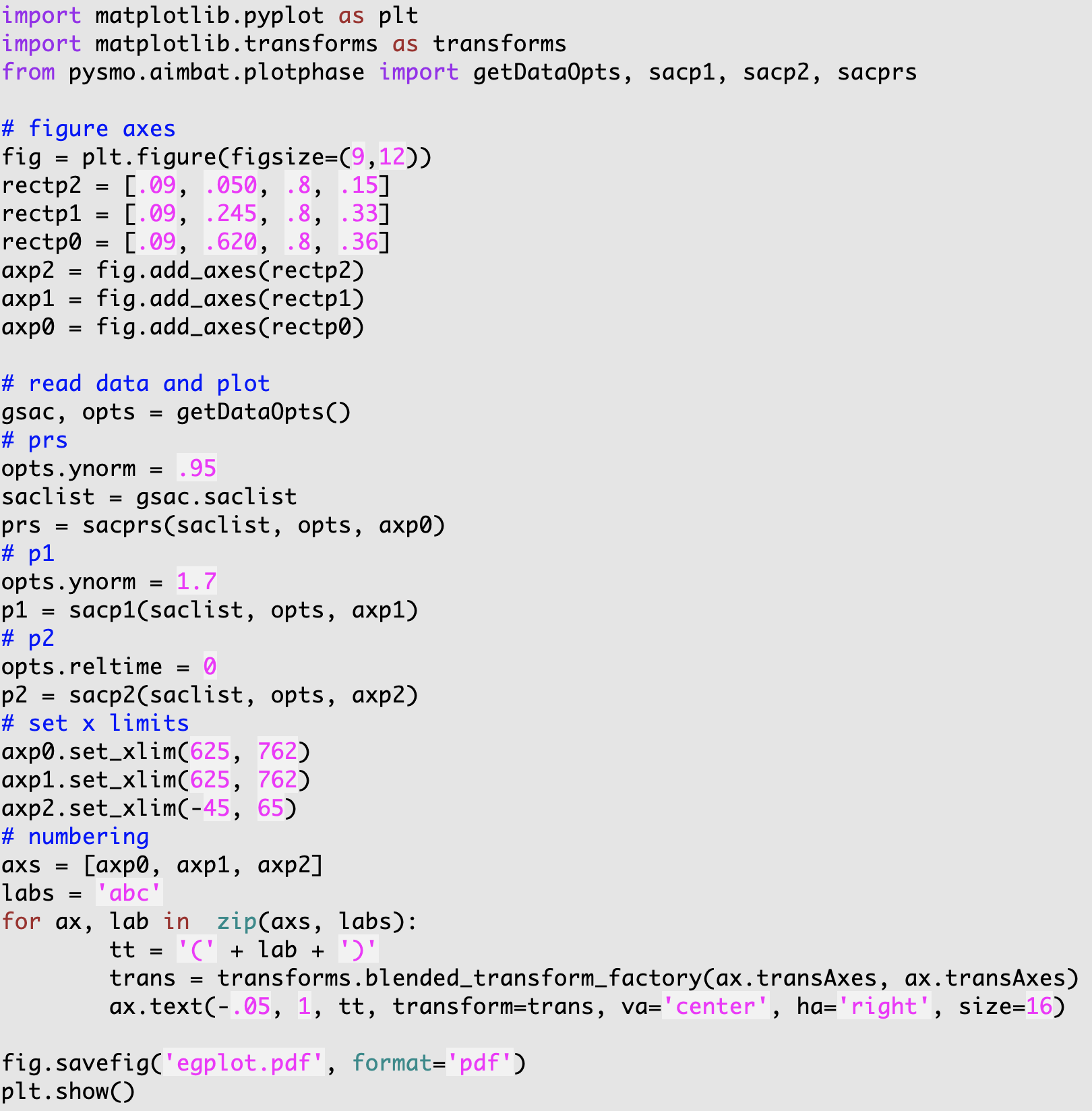
Besides using the standard aimbat-sacplot script, the user can modify its getAxes function in their own script to customize figure size and axes attributes. Script egplot.py is such an example in which SAC p1, p2 styles and record section plotting are drawn in three axes in the same figure canvas. Run:

egplot.py TA.[1-K]*Z  -f1 -C

at command line to produce the figure below.

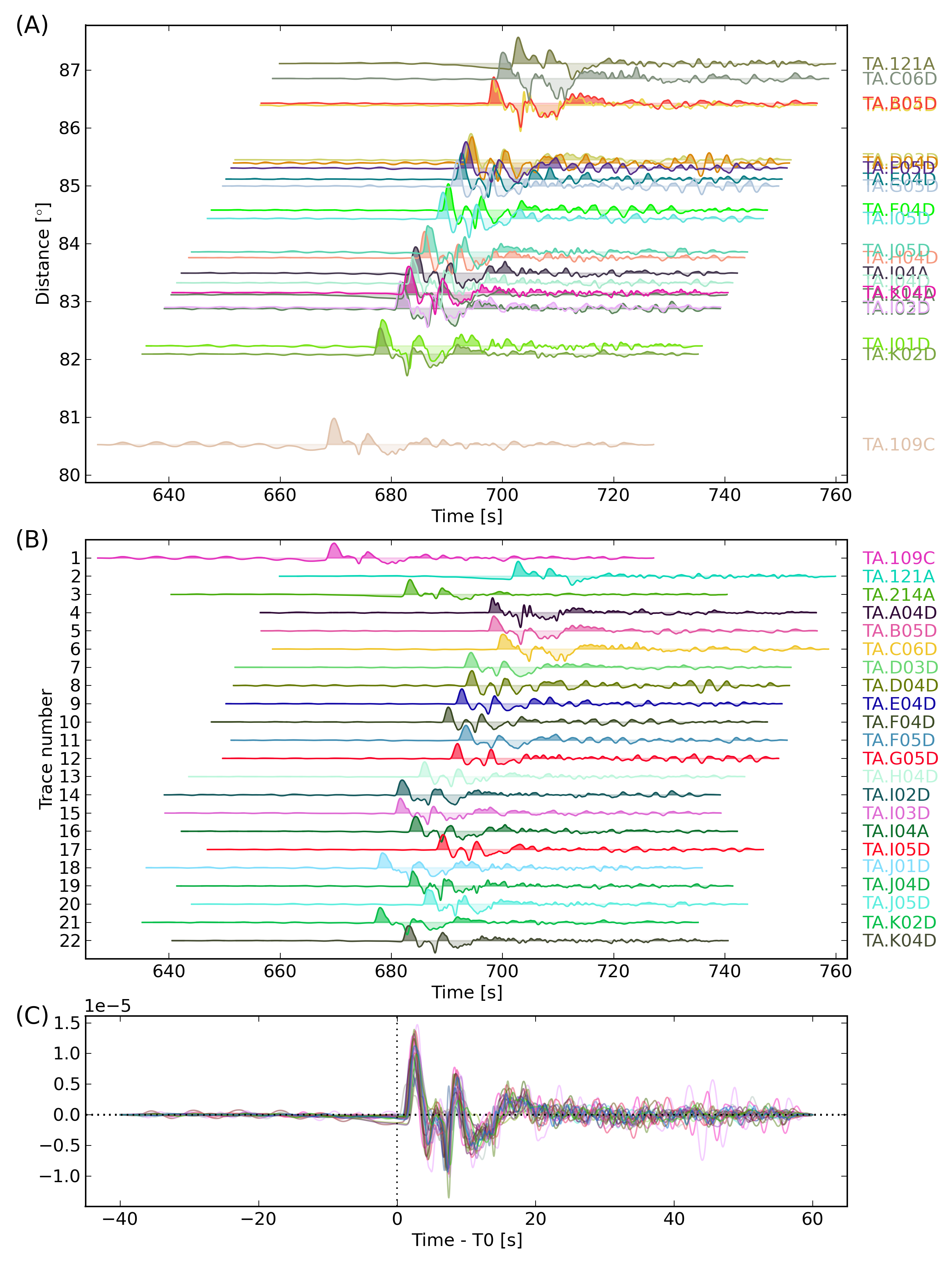
The “-C” option uses random color for each seismogram. The “-f1” option fills the positive signals of waveform with less transparency. In the script, “opts.ynorm” sets the waveform normalization and “opts.reltime=0” sets the time axis relative to time pick t0.

An improvement over SAC is that the program outputs the filename when the seismogram is clicked on by the mouse. This is enabled by the event handling API and is mostly introduced for use in SAC p2 style plotting when seismograms are plotted on top of each other. It is especially useful when a large number of seismograms create difficulties in labeling.

Another improvement is easier window zooming enabled by the SpanSelector widget and the event handling API. Select a time span by mouse clicking and dragging to zoom in a waveform section. Press the ‘z’ key to zoom out to the previous time range.

3.5. SAC Phase Picking

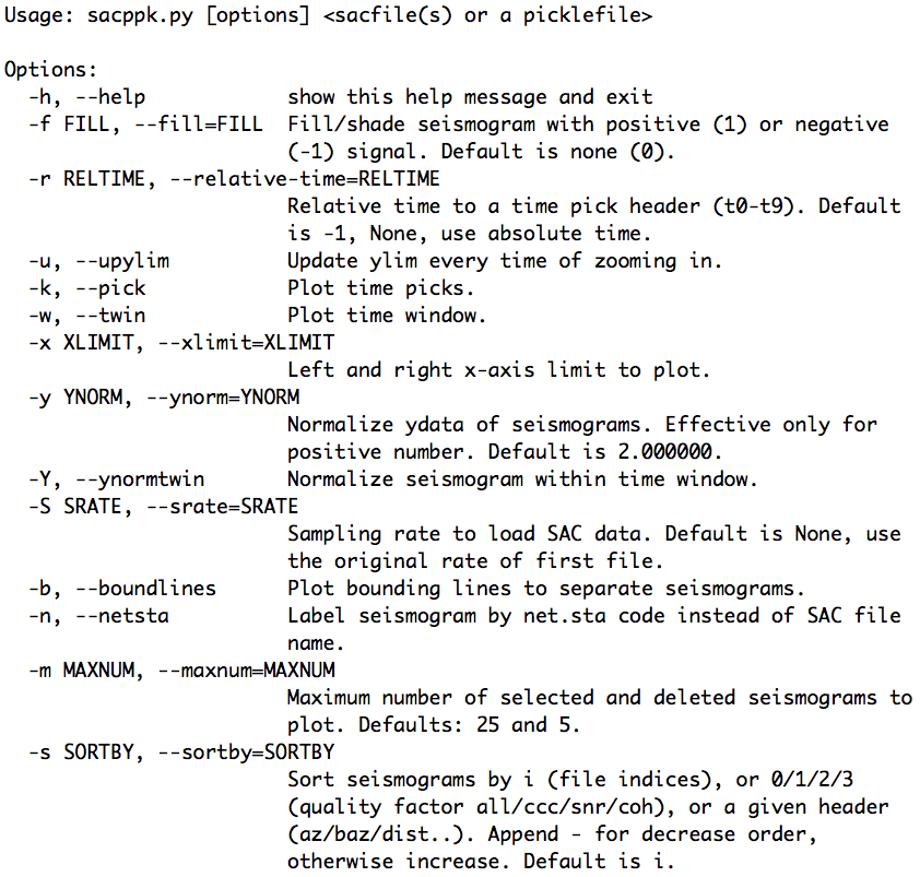
SAC plotting (pysmo.aimbat.plotphase) does not involve change in data files, but phase picking (pysmo.aimbat.pickphase) does. A GUI is built for the user to interactively pick phase arrival times. The figure below is an example screen shot running:

aimbat-sacppk 20110915.19310408.bhz.pkl -w

in the data example directory <example-event-dir>.

Following SAC convention, the user can set a time pick by pressing the ‘t’ key and number keys ‘0-9’. The x location of the mouse position is saved to corresponding SAC headers ‘t0-t9’. Time window zooming in pysmo.aimbat.pickphase is implemented in the same way as in pysmo.aimbat.plotphase to replace SAC’s combination of the ‘x’ key and mouse click. Zooming out key is set to ‘z’ because the ‘o’ key is used for another purpose by Matplotlib. The filename printing out by mouse clicking feature is also available in pysmo.aimbat.pickphase.

A major improvement over SAC is picking a time window in addition to time picks. Pressing the ‘w’ key to save the current time axis range to two user-defined SAC header variables. A transparent green span is plotted within the time window, as shown in the figure below.

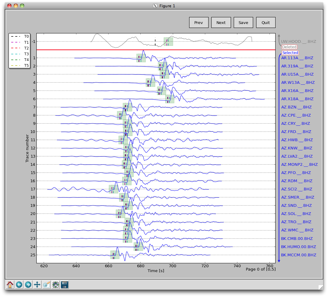
Another major improvement involves quality control with convenient operations to (de)select seismograms. In the GUI above, there are two divisions of selected and deleted seismograms. Selected seismograms with a positive trace number are displayed with blue wiggles, while deleted seismograms with negative trace numbers are plotted in gray. The user can simply click on a certain seismogram to switch the selection status, either to exclude it or bring it back for inclusion. The trace selection status is stored in a user-defined SAC header variable.

In SAC, command ppk p 10 plots 10 seismograms on each page. Pressing the ‘b’ and ‘n’ keys to navigate through pages. The number of seismograms plotted on each page is controlled by command line option:

-m maxsel maxdel

for aimbat-sacppk. The Prev and Next buttons are for page navigation and the Save Button saves the change in time picks and time window to files. The default values for maxsel and maxdel are 25 and 5, which means a maximum of 30 seismograms on each page.

In the figure displayed, there are 26 seismograms on the first page because only 1 seismogram is deleted. On the next page, there are 30 selected seismograms. To plot 50 seismograms on each page, run:

aimbat-sacppk 20110915.19310408.bhz.pkl -w -m 45 5

and there would be 4 total pages and 13 seismograms on the last page.

To plot seismograms relative to time pick t0 and fill the positive and negative wiggles of waveform, run:

aimbat-sacppk 20110915.19310408.bhz.pkl -w -r0 -f1

To sort seismograms by epicentral distance in increase and decrease orders, run:

aimbat-sacppk 20110915.19310408.bhz.pkl -w -sdist
aimbat-sacppk 20110915.19310408.bhz.pkl -w -sdist-

Sorting by azimuth and back-azimuth is similar:

aimbat-sacppk 20110915.19310408.bhz.pkl -w -saz
aimbat-sacppk 20110915.19310408.bhz.pkl -w -sbaz

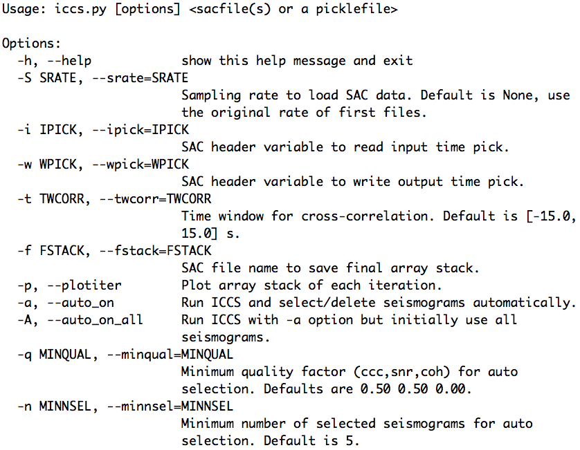
The help message of the aimbat-iccs script is shown below:

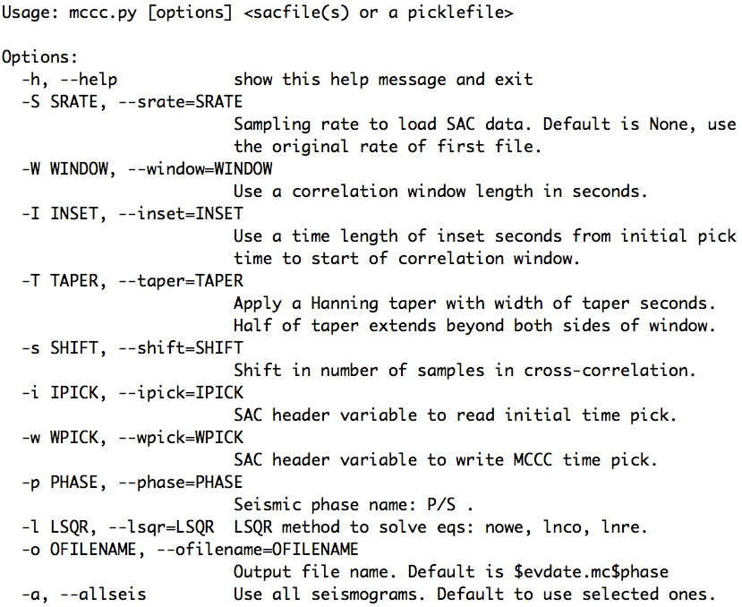
The help message of the aimbat-mccs script is shown below:

3.6. Measuring Teleseismic Body Wave Arrival Times

The core idea in using AIMBAT to measure teleseismic body wave arrival times has two parts:

automated phase alignment, to reduce user processing time, and
interactive quality control, to retain valuable user inputs.

3.6.1. Automated Phase Alignment

The ICCS algorithm calculates an array stack from predicted time picks, cross-correlates each seismogram with the array stack to find the time lags at maximum cross-correlation, then uses the new time picks to update the array stack in an iterative process. The MCCC algorithm cross-correlates each possible pair of seismograms and uses a least-squares method to calculate an optimized set of relative arrival times. Our method combines ICCS and MCCC in a four-step procedure using four anchoring time picks \(_0T_i,\,_1T_i,\,_2T_i,\) and \(_3T_i\).

Coarse alignment by ICCS
Pick phase arrival at the array stack
Refined alignment by ICCS
Final alignment by MCCC

The one-time manual phase picking at the array stack in step (b) allows the measurement of absolute arrival times. The detailed methodology and procedure can be found in [LouVanDerLee2013].

Time picks and their SAC headers used in the procedure for measuring teleseismic body wave arrival times.
Step	Algorithm	Input			Output
Step	Algorithm	Time Window	Time Pick	Time Header	Time Pick	Time Header
	ICCS	\(W_a\)	\(_0T_i\)	T0	\(_1T_i\)	T1
	ICCS	\(W_b\)	\(_2T'_i\)	T2	\(_2T_i\)	T2
	MCCS	\(W_b\)	\(_2T_i\)	T2	\(_3T_i\)	T3

The ICCS and MCCC algorithms are implemented in two modules pysmo.aimbat.algiccs and pysmo.aimbat.algmccc, and can be executed in scripts iccs.py and mccc.py respectively.

3.6.2. Picking Travel Times

This section explains how to run the program aimbat-ttpick to get the travel times you want.

3.6.2.1. Getting into the right directory

In the terminal, cd into the directory with all of the pkl files you want to run. You want to run either the BHT or BHZ files. BHT files are for S-waves and BHZ files are for P-waves. PKL is a bundle of SAC files. Each SAC file is a seismogram, but since there may be many seismograms from various stations for each event, we bundle them into a PKL file so we only have to import one file into AIMBAT, not a few hundred of them.

3.6.2.2. Running aimbat-ttpick

Run aimbat-ttpick -p P <path-to-pkl-file> for BHZ files or aimbat-ttpick -p S <path-to-pkl-file> for BHT files. A GUI should pop up if you successfully ran it. Note that if you click on the buttons, they will not work until you move your mouse off them; this is a problem we are hoping to fix.

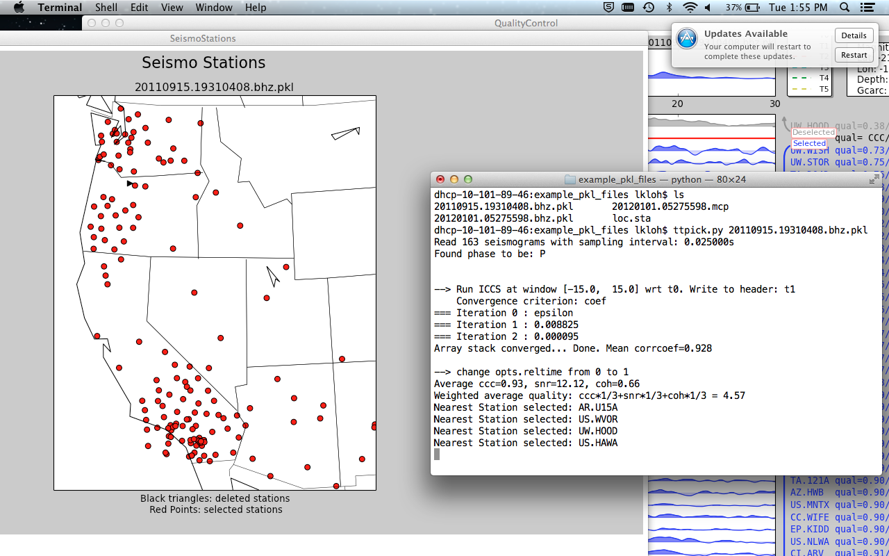
You can get some example data to test this out by downloading the Github repository data-example. Now, cd into the folder example_pkl_files, which has several pickle files for seismic events. Type:

aimbat-ttpick -p P 20110915.19310408.bhz.pkl

and a python GUI should pop up.

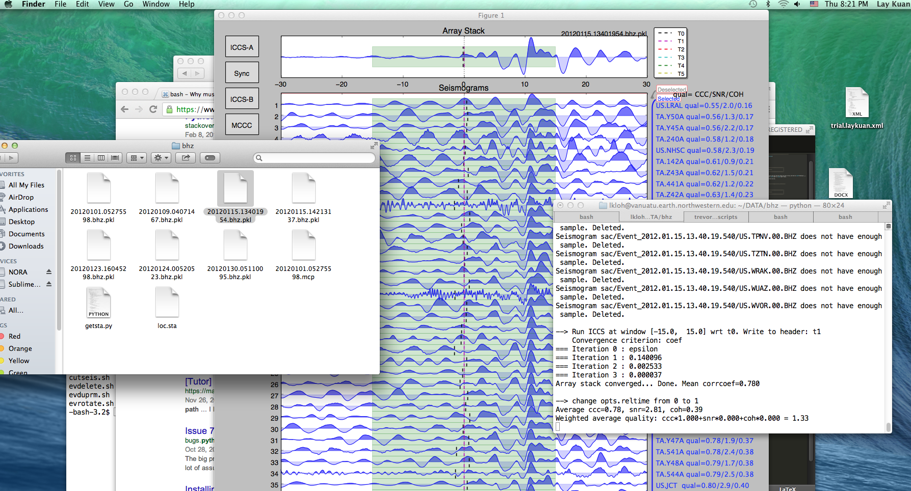
At the top of the GUI is the scaled sum of all of the seismograms known as the array stack, which gives a characteristic waveform of the event for the stations involved. Beneath this is a page of seismograms, with the corresponding station and various quality factors listed on the right. CCC is the cross-correlation coefficient between that seismogram and the array stack, SNR is the signal-to-noise ratio, and COH is the coherence between that seismogram and the array stack.

3.6.2.3. Initial deselection of bad seismograms

Bad seismograms are those whose waveforms look nothing like the array stack above. By default, the seismograms are sorted by quality, so bad seismograms will likely be at the top. In order to deselect these, click on the waveforms themselves (not the fill) and wait a second or two for them to turn gray. The user can develop criteria for which seismograms to deselect and which to keep. Simply deselecting all seismograms below a certain quality threshold can decrease time but may lead to good seismograms being deselected or bad seismograms remaining.

Remember to save your work periodically once you start picking your travel times. Otherwise, if AIMBAT crashes, you will lose your work.

3.6.2.4. Align

The first step after deselecting seismograms is to press Align. This will recalculate both the array stack and the T1 picks for the seismograms, not including the deselected seismograms. Do not press Align after pressing Sync unless you wish to remove any T2 picks that have been made.

3.6.2.5. Sync, refine, and setting time window

After hitting the Align button, place the cursor on the array stack where the first motion of the seismogram, either up or down, occurs. Press t and 2 simultaneously on the keyboard to select the arrival time. Now press Sync. Use the mouse to drag and select the desired time window on the seismogram on the array stack. This time window is the portion of the seismogram on which cross-correlation will be run. The time window should begin 2-10 seconds before the first arrival and include a few seconds of the first motion of the waveform. The final time window should be smaller than the default window to increase the accuracy of the cross-correlation.

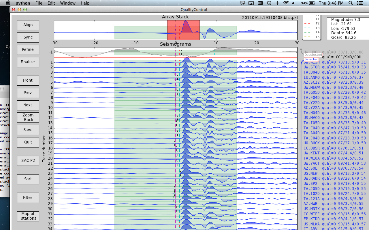
_images/selecting-time-window-highlight.png

Next, set the cursor over the array stack and press the w key. If the new time window has been saved, a message noting the new size of the time window will be printed in the terminal. The entire width of the x-axis is now colored green and will be stored as the time window to use for the cross-correlations. Press Save headers only if you wish to keep this time window for future applications.

Now press Refine and all the seismograms will align with the smaller time window. Note that the Weighted average quality printed to the terminal may decrease significantly, but this is likely due to the fact that the time window is smaller than the original.

3.6.2.6. Filtering

If you wish to apply a filter to your data, hit the Filter button, and a window will pop up for you to use the Butterworth filter to filter your data.

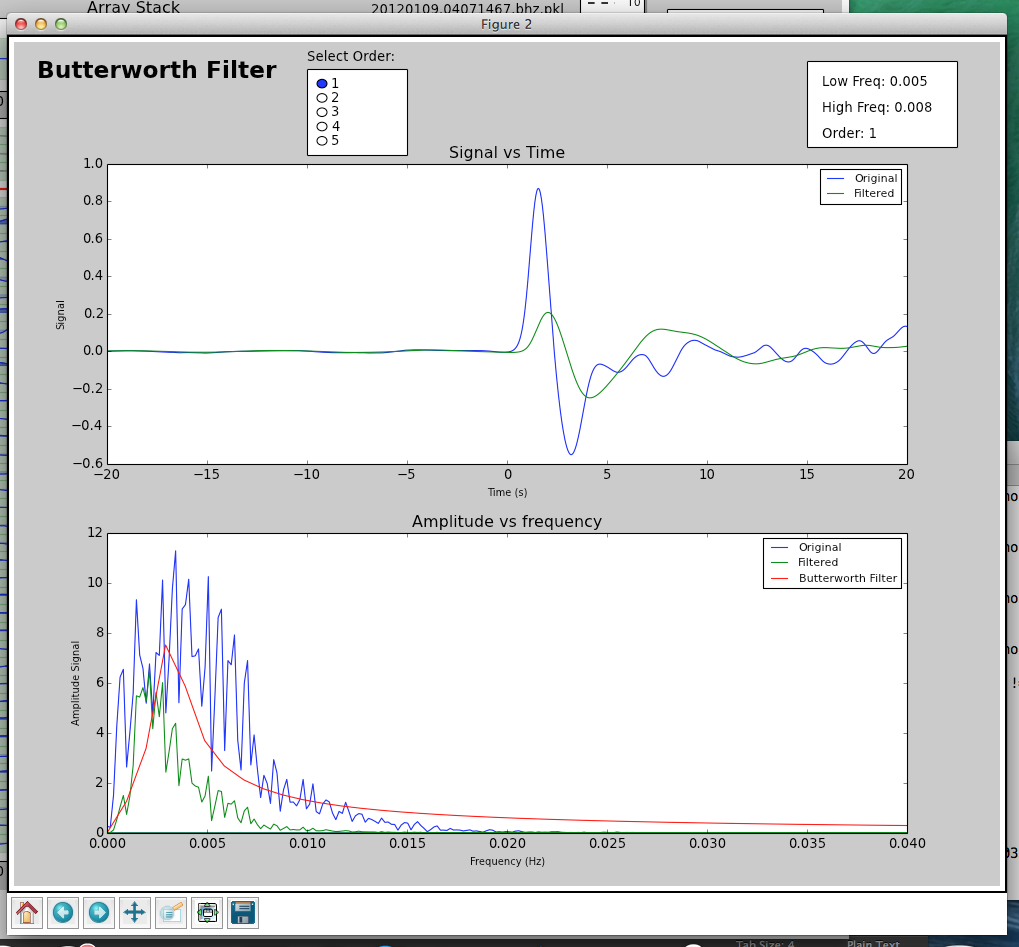
The defaults used for filtering are:

Variable	Default
Order	2
Filter Type	Bandpass
Low Frequency	0.05 Hz
High Frequency	0.25 Hz

You can change the order and filter type by selecting the option you want. In order to set corner frequencies for the filter, select the low frequency and the high frequency you want on the lower figure by clicking. Press Apply to filter the seismograms when you are satisfied with the filter parameters chosen.

3.6.2.7. Finalize

Hit Finalize to run the multi-channel cross-correlation. Do not hit Align or Refine again, or all your previous picks will be written over. A warning will pop up to check if you really do want to hit these two buttons if you do click on them.

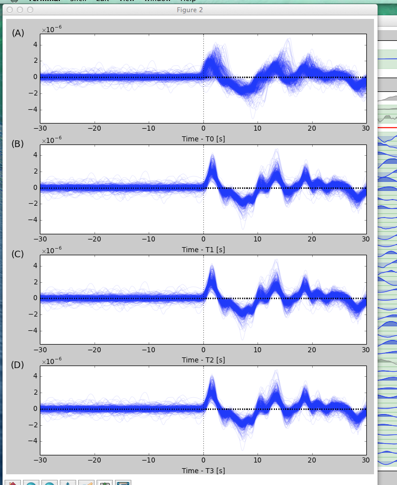
3.6.2.8. SACP2 to check for outlier seismograms

Hit SACP2 and go to the last figure, (d). Zoom in to have a better look. Zooming in doesn’t always work well; close and reopen the SACP2 window if there are problems.

Click on the outliers that stray from the main group of stacked seismograms. The terminal will output the names of the seismograms that you clicked on, so you can return to the main GUI window and readjust the travel times. Note: hitting SACP2 before hitting Finalize will often cause AIMBAT to close, so make sure you have finalized before using SACP2.

3.6.2.9. Go through the badly aligned seismograms and realign the travel times manually

By default, the worst seismograms are on the first page, and as you click through the pages, the quality of the seismograms gradually gets better. Keep using t2 to realign the arrival times so that the peaks of all the seismograms are nicely aligned. Remember to zoom in to have a better look.

However, you may wish to sort the seismograms in alphabetical order or by azimuth so that you can find the bad seismogrrams and correct them more easily. Hit the Sort button and a window will pop up for you to choose which sorting method to use. In this case, choose File to sort the files by station name alphabetically, or choose AZ to sort the files by azimuth from the event epicenter. The seismograms are stretched to fit together, but they may be scaled differently.

3.6.3. What the Alignments Stand For

T0: Theoretical Arrival
T1: Pick from initial cross correlation
T2: Travel Time pick
T3: MCCC pick
T4: Zoom in

3.6.4. Post Processing

3.6.4.1. Getting the output

In the same folder as the initial PKL file you ran aimbat-ttpick on, you can find the output list with extension <event name>.mcp, which contains the travel time arrivals.

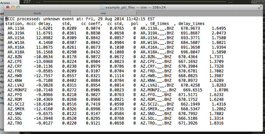
mccc delay is t3+average arrival times, and t0_times are the theoretical arrival times. delay_times are obtained by taking t3-t0.

3.6.4.2. Disclaimer about delay times

t0 depends on hypocenter location, origin time, and reference model. We compute the delay time by finding t3-t0, but it does not have elliptic, topological, or crust corrections.

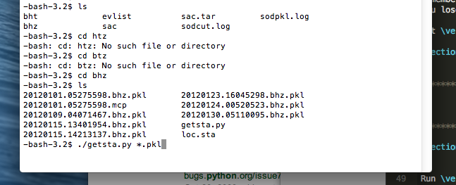
3.6.4.3. Getting the stations of the seismograms chosen

Run getsta.py in the additional scripts (not on Github for now). It gives the unique list of stations where the seismograms came from. You need to run it with the list of all pkl files chosen after you saved to. To do this, type ./getsta.py *.pkl.

3.6.4.4. Visualizing Stations on a map

After running:

aimbat-ttpick <sac-files>

Hit Map of Stations in order to get a visual respresentation of where exactly each station is. Dots represent circles used for computing delay times; black triangles represent discarded stations. Click on a dot to get the station name in the terminal.

3.6.5. Picking Travel Times does not work

If you run aimbat-ttick <Event name>.bhz.pkl, a GUI will pop up for you to manually pick the travel times by pressing the keyboard. If typing on the keyboard as directed does not allow you to pick travel times, it could be a problem with the keyboard settings, or the matplotlib backend.

To fix this, first look for the .matplotlib directory. It is hidden in your home directory, so do ls -a to find it.

Once you have found the .matplotlib directory, cd into it, and then look for the matplotlibrc file. Inside that file, ensure the backend is set to:

backend : TkAgg

Make sure to comment out the other backends.

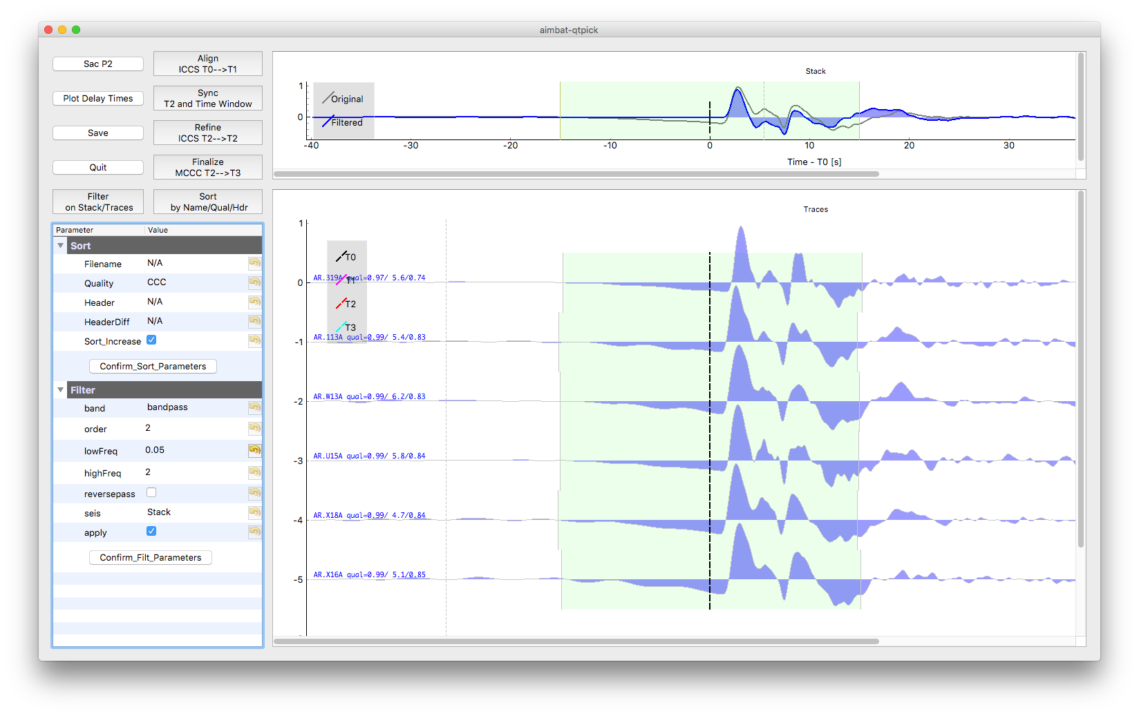
3.7. Alternative Qt GUI for Measuring Arrival Times

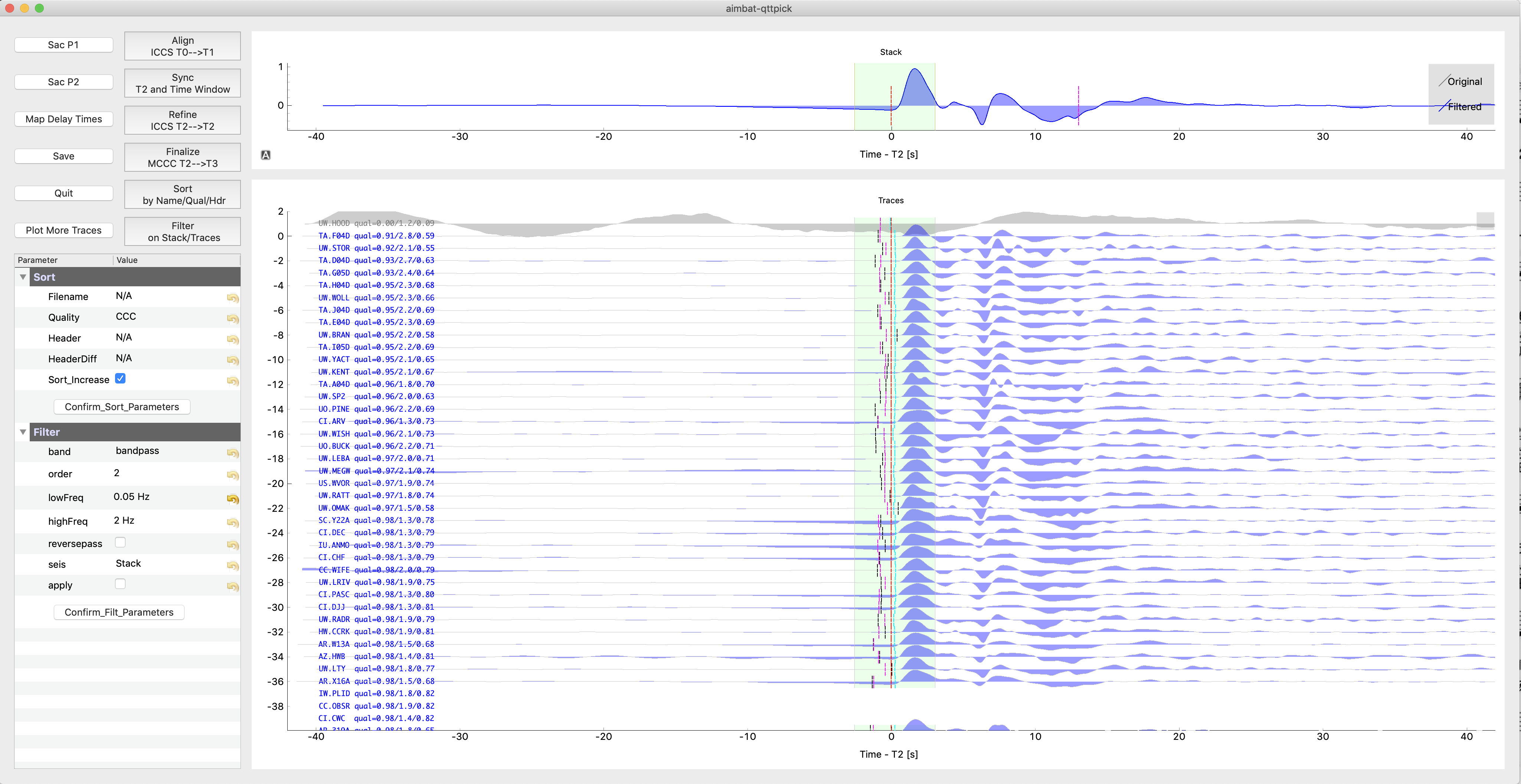
The Matplotlib GUI is slow for interactive plotting. An additional GUI based on pyqtgraph was built since v1.0.0 to speed up plotting. Similar to the old GUI, run:

aimbat-qttpick <path-to-pkl-file>

to launch the Qt GUI. Phase of the seismogram (P or S), if not given in command line, can be automatically found based on file names including BHZ or BHT. Here is aGn example snapshot:

The AIMBAT philosophy of using the five-step (Align, Pick, Sync, Refine, and Finalize) procedure for automated and interactive phase arrival time measurement is the same.

Some GUI behavior remains the same:

the phase picking steps of Align, Pick, Sync, Refine, and Finalize.
mouse clicking waveforms to change trace selection status.
keyboard interaction: t[0-9] to pick time, and w to set time window.
Click Button Sac P2 to overlay all traces relative to time picks

Some components are different:

Choose sort and filter options in a parameter tree and apply in the same GUI window.
All traces plotted in one long page, instead of multiple pages.
Still Possible to plot a subset of traces. Click button to add more traces to the plotting window.
Pyqtgraph mouse events: e.g., right mouse button drag to zoom in and out.
Time window is plotted as a pyqtgraph.LinearRegionItem instead of Matplotlib Span Selector. To change time window size, just drag either side line and move. Still press key w to set time window.
A vertical hair indicating the time axis value is always plotted follow the mouse movement.

In the above example, 37 selected seismograms are plotted initially. During the arrival time measurement procedure, traces sorting order is changed after time window size or sorting parameters are changed. Trace 37, 38, 39 are missing in the GUI. You can optionally click Plot More Traces Button to fill the gap. You can also zoom out vertically and plot more traces.

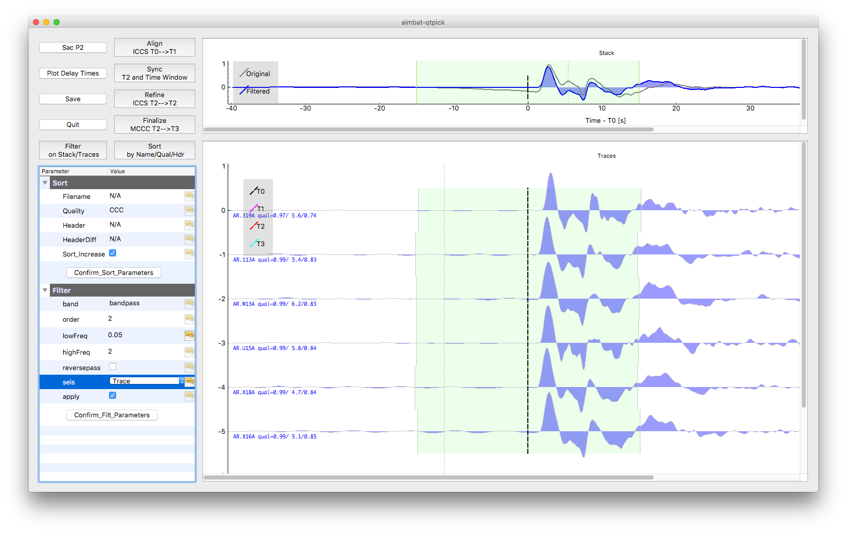
Here is an example of filtering seismograms. First choose filtering parameters in the parameter tree and test on the stack by clicking Button Confirm_Filt_Parameters and Button Filter on Stack/Traces. Then applied filter to traces after parameters are finalized.

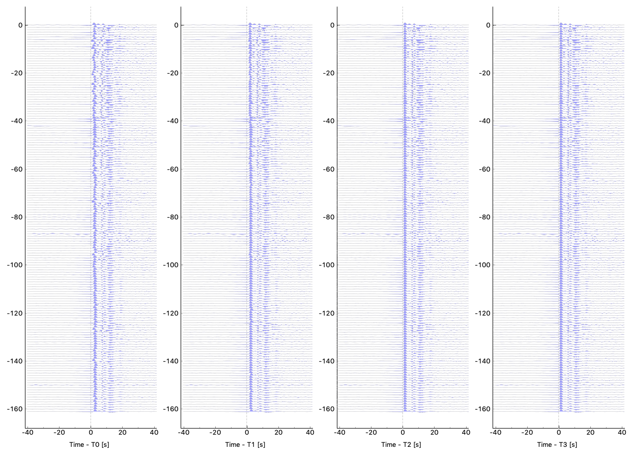
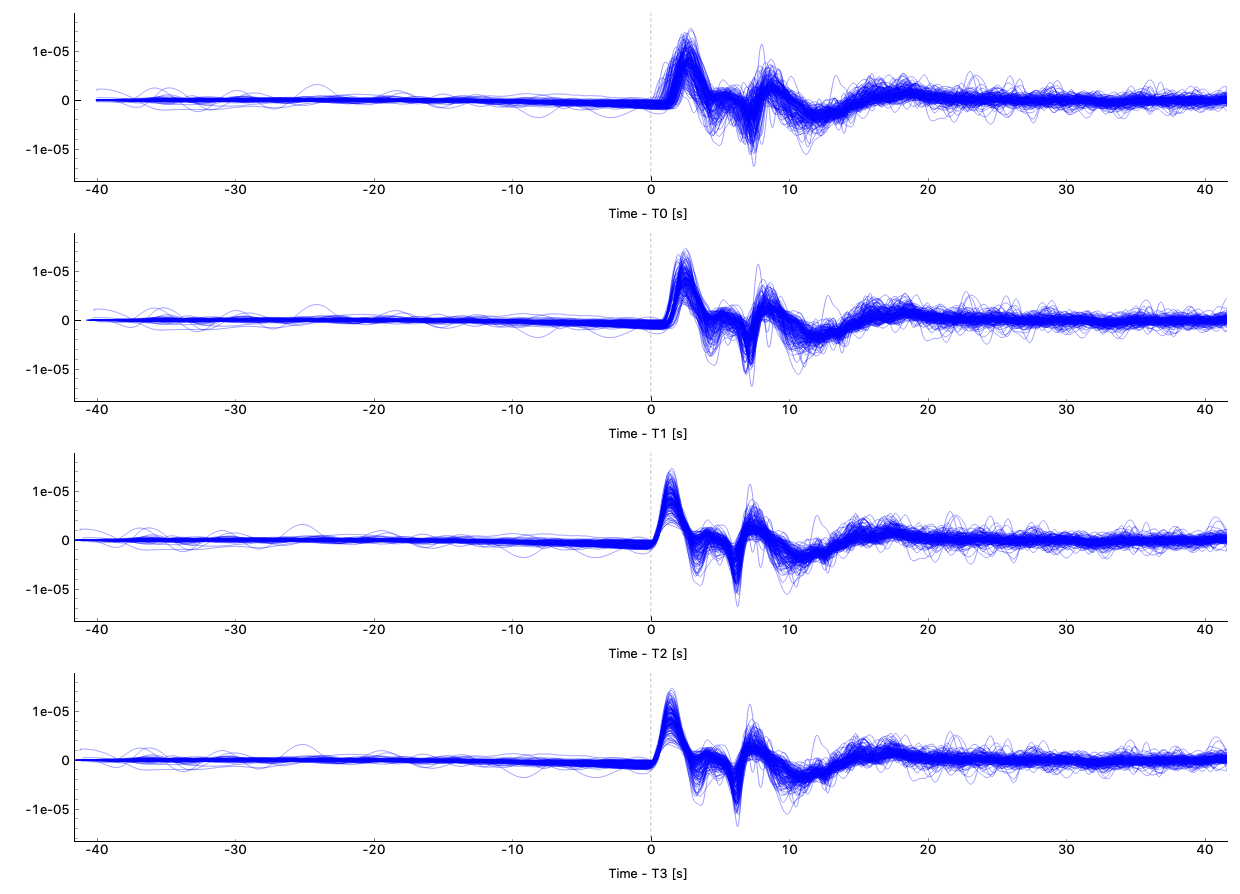
Some QC tools are available in this Qt GUI. Click Button Sac P1 and Sac P2 to plot traces relative to four time picks T0, T1, T2, and T3. Click Button Plot Delay Times to plot absolute delay times in a map view.

More details might be added here in the future.